solve

S = solve( eqn , var ) solves the symbolic equation eqn for the variable var . If you do not specify var , the symvar function determines the variable to solve for. For example, solve(x + 1 == 2, x) solves the equation x + 1 = 2 for x.

S = solve( eqn , var , Name=Value ) uses additional options specified by one or more Name=Value arguments.

Y = solve( eqns , vars ) solves the system of equations eqns for the variables vars and returns a structure that contains the solutions. If you do not specify vars , solve uses symvar to find the variables to solve for. In this case, the number of variables that symvar finds is equal to the number of equations eqns .

Y = solve( eqns , vars , Name=Value ) uses additional options specified by one or more Name=Value arguments.

[ y1. yN ] = solve( eqns , vars ) solves the system of equations eqns for the variables vars . The solutions are assigned to the variables y1. yN . If you do not specify the variables, solve uses symvar to find the variables to solve for. In this case, the number of variables that symvar finds is equal to the number of output arguments N .

[ y1. yN ] = solve( eqns , vars , Name=Value ) uses additional options specified by one or more Name=Value arguments.

[ y1. yN , parameters , conditions ] = solve( eqns , vars ,ReturnConditions=true) returns the additional arguments parameters and conditions that specify the parameters in the solution and the conditions on the solution.

Examples

Solve Quadratic Equation

Solve the quadratic equation without specifying a variable to solve for. solve chooses x to return the solution.

syms a b c x eqn = a*x^2 + b*x + c == 0

eqn = $$a{x}^2+bx+c=0$$

S = solve(eqn)

S = 
$$\left(\begin{array}{c}-\frac{b+\sqrt{b^2-4ac}}{2a}\\ -\frac{b-\sqrt{b^2-4ac}}{2a}\end{array}\right)$$

Specify the variable to solve for and solve the quadratic equation for a .

Sa = solve(eqn,a)

Sa = 
$$-\frac{c+bx}{x^2}$$

Solve Polynomial and Return Real Solutions

Solve a fifth-degree polynomial. It has five solutions.

syms x eqn = x^5 == 3125; S = solve(eqn,x)

S = 
$$\begin{array}{l}\left(\begin{array}{c}5\\ -{\sigma }_1-\frac{5}{4}-\frac{5\sqrt{2}\sqrt{5-\sqrt{5}}\mathrm{i}}{4}\\ -{\sigma }_1-\frac{5}{4}+\frac{5\sqrt{2}\sqrt{5-\sqrt{5}}\mathrm{i}}{4}\\ {\sigma }_1-\frac{5}{4}-\frac{5\sqrt{2}\sqrt{\sqrt{5}+5}\mathrm{i}}{4}\\ {\sigma }_1-\frac{5}{4}+\frac{5\sqrt{2}\sqrt{\sqrt{5}+5}\mathrm{i}}{4}\end{array}\right)\\ \\ \mathrm{where}\\ \\ {\sigma }_1=\frac{5\sqrt{5}}{4}\end{array}$$

Return only real solutions by setting the Real argument to true . The only real solutions of this equation is 5 .

S = solve(eqn,x,Real=true)

S = $$5$$

Numerically Solve Equations

When solve cannot symbolically solve an equation, it tries to find a numeric solution using vpasolve . The vpasolve function returns the first solution found.

Try solving the following equation. solve returns a numeric solution because it cannot find a symbolic solution.

syms x eqn = sin(x) == x^2 - 1; S = solve(eqn,x)

S = $$-0.63673265080528201088799090383828$$

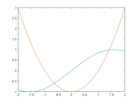
Plot the left and the right sides of the equation. Observe that the equation also has a positive solution.

fplot([lhs(eqn) rhs(eqn)], [-2 2])

Find the other solution by directly calling the numeric solver vpasolve and specifying the interval.

V = vpasolve(eqn,x,[0 2])

V = $$1.4096240040025962492355939705895$$

Solve Multivariate Equations and Assign Outputs to Structure

When solving for multiple variables, it can be more convenient to store the outputs in a structure array than in separate variables. The solve function returns a structure when you specify a single output argument and multiple outputs exist.

Solve a system of equations to return the solutions in a structure array.

syms u v eqns = [2*u + v == 0, u - v == 1]; S = solve(eqns,[u v])

S = struct with fields: u: 1/3 v: -2/3

Access the solutions by addressing the elements of the structure.

ans = 
$$\frac{1}{3}$$

ans = 
$$-\frac{2}{3}$$

Using a structure array allows you to conveniently substitute solutions into other expressions.

Use the subs function to substitute the solutions S into other expressions.

expr1 = u^2; e1 = subs(expr1,S)

e1 = 
$$\frac{1}{9}$$

expr2 = 3*v + u; e2 = subs(expr2,S)

e2 = 
$$-\frac{5}{3}$$

If solve returns an empty object, then no solutions exist.

eqns = [3*u+2, 3*u+1]; S = solve(eqns,u)

S = Empty sym: 0-by-1

Solve Inequalities

The solve function can solve inequalities and return solutions that satisfy the inequalities. Solve the following inequalities.

Set ReturnConditions to true to return any parameters in the solution and conditions on the solution.

syms x y eqn1 = x > 0; eqn2 = y > 0; eqn3 = x^2 + y^2 + x*y < 1; eqns = [eqn1 eqn2 eqn3]; S = solve(eqns,[x y],ReturnConditions=true); S.x

ans = 
$$\frac{\sqrt{u-3v^2}}{2}-\frac{v}{2}$$

ans = $$v$$

S.parameters

ans = $$\left(\begin{array}{cc}u& v\end{array}\right)$$

S.conditions

ans = $$4v^2<mi>u</mi>\wedge u<mn>4</mn>\wedge 0<mi>v</mi>$$

The parameters u and v do not exist in MATLAB® workspace and must be accessed using S.parameters .

Check if the values u = 7/2 and v = 1/2 satisfy the condition using subs and isAlways .

condWithValues = subs(S.conditions, S.parameters, [7/2,1/2]); isAlways(condWithValues)

ans = logical 1

isAlways returns logical 1 ( true ) indicating that these values satisfy the condition. Substitute these parameter values into S.x and S.y to find a solution for x and y .

xSol = subs(S.x, S.parameters, [7/2,1/2])

xSol = 
$$\frac{\sqrt{11}}{4}-\frac{1}{4}$$

ySol = subs(S.y, S.parameters, [7/2,1/2])

ySol = 
$$\frac{1}{2}$$

Solve Multivariate Equations and Assign Outputs to Variables

Solve the system of equations.

When solving for more than one variable, the order in which you specify the variables defines the order in which the solver returns the solutions. Assign the solutions to variables solv and solu by specifying the variables explicitly. The solver returns an array of solutions for each variable.

syms u v eqns = [2*u^2 + v^2 == 0, u - v == 1]; vars = [v u]; [solv, solu] = solve(eqns,vars)

solv = 
$$\left(\begin{array}{c}-\frac{2}{3}-\frac{\sqrt{2}\mathrm{i}}{3}\\ -\frac{2}{3}+\frac{\sqrt{2}\mathrm{i}}{3}\end{array}\right)$$

solu = 
$$\left(\begin{array}{c}\frac{1}{3}-\frac{\sqrt{2}\mathrm{i}}{3}\\ \frac{1}{3}+\frac{\sqrt{2}\mathrm{i}}{3}\end{array}\right)$$

Entries with the same index form the pair of solutions.

solutions = [solv solu]

solutions = 
$$\left(\begin{array}{cc}-\frac{2}{3}-\frac{\sqrt{2}\mathrm{i}}{3}& \frac{1}{3}-\frac{\sqrt{2}\mathrm{i}}{3}\\ -\frac{2}{3}+\frac{\sqrt{2}\mathrm{i}}{3}& \frac{1}{3}+\frac{\sqrt{2}\mathrm{i}}{3}\end{array}\right)$$

Use Parameters and Conditions to Refine Solution

Return the complete solution of an equation with parameters and conditions of the solution by specifying ReturnConditions as true .

Solve the equation sin ( x ) = 0 . Provide two additional output variables for output arguments parameters and conditions .

syms x eqn = sin(x) == 0; [solx,parameters,conditions] = solve(eqn,x,ReturnConditions=true)

solx = $$\pi k$$

parameters = $$k$$

conditions = $$k\in \mathbb{Z}$$

The solution π k contains the parameter k , where k must be an integer. The variable k does not exist in the MATLAB® workspace and must be accessed using parameters .

assume(conditions) restriction = [solx > 0, solx < 2*pi]; solk = solve(restriction,parameters)

solk = $$1$$

valx = subs(solx,parameters,solk)

valx = $$\pi$$

Alternatively, determine the solution for x by choosing a value of k . Check if the value chosen satisfies the condition on k using isAlways .

Check if k = 4 satisfies the condition on k .

condk4 = subs(conditions,parameters,4); isAlways(condk4)

ans = logical 1

isAlways returns logical 1( true ), meaning that 4 is a valid value for k . Substitute k with 4 to obtain a solution for x . Use vpa to obtain a numeric approximation.

valx = subs(solx,parameters,4)

valx = $$4\pi$$

vpa(valx)

ans = $$12.5664$$

Shorten Result with Simplification Rules

Solve the equation exp ( log ( x ) log ( 3 x ) ) = 4 .

By default, solve does not apply simplifications that are not valid for all values of x . In this case, the solver does not assume that x is a positive real number, so it does not apply the logarithmic identity log ( 3 x ) = log ( 3 ) + log ( x ) . As a result, solve cannot solve the equation symbolically.

syms x eqn = exp(log(x)*log(3*x)) == 4; S = solve(eqn,x)

S = $$-14.009379055223370038369334703094-2.9255310052111119036668717988769\mathrm{i}$$

Set IgnoreAnalyticConstraints to true to apply simplification rules that might allow solve to find a solution. For details, see Algorithms.

S = solve(eqn,x,IgnoreAnalyticConstraints=true)

S = 
$$\left(\begin{array}{c}\frac{\sqrt{3}{\mathrm{e}}^{-\frac{\sqrt{\log \left(256\right)+{\log \left(3\right)}^2}}{2}}}{3}\\ \frac{\sqrt{3}{\mathrm{e}}^{\frac{\sqrt{\log \left(256\right)+{\log \left(3\right)}^2}}{2}}}{3}\end{array}\right)$$

solve applies simplifications that allow the solver to find a solution. The mathematical rules applied when performing simplifications are not always valid in general. In this example, the solver applies logarithmic identities with the assumption that x is a positive real number. Therefore, the solutions found in this mode should be verified.

Ignore Assumptions on Variables

The sym and syms functions let you set assumptions for symbolic variables.

Assume that the variable x is positive.

syms x positive

When you solve an equation for a variable under assumptions, the solver only returns solutions consistent with the assumptions. Solve this equation for x .

eqn = x^2 + 5*x - 6 == 0; S = solve(eqn,x)

S = $$1$$

Allow solutions that do not satisfy the assumptions by setting IgnoreProperties to true .

S = solve(eqn,x,IgnoreProperties=true)

S = 
$$\left(\begin{array}{c}-6\\ 1\end{array}\right)$$

For further computations, clear the assumption that you set on the variable x by recreating it using syms .

syms x

Solve Polynomial Equations of High Degree

When you solve a polynomial equation, the solver might use root to return the solutions. Solve a third-degree polynomial.

syms x a eqn = x^3 + x^2 + a == 0; solve(eqn, x)

ans = 
$$\left(\begin{array}{c}\mathrm{root}\left(z^3+z^2+a,z,1\right)\\ \mathrm{root}\left(z^3+z^2+a,z,2\right)\\ \mathrm{root}\left(z^3+z^2+a,z,3\right)\end{array}\right)$$

Try to get an explicit solution for such equations by calling the solver with MaxDegree argument. This argument specifies the maximum degree of polynomials for which the solver tries to return explicit solutions. The default value is 2 . Increasing this value, you can get explicit solutions for higher order polynomials.

Solve the same equations for explicit solutions by increasing the value of MaxDegree to 3 .

S = solve(eqn,x,MaxDegree=3)

S = 
$$\begin{array}{l}\left(\begin{array}{c}\frac{1}{9{\sigma }_1}+{\sigma }_1-\frac{1}{3}\\ -\frac{1}{18{\sigma }_1}-\frac{{\sigma }_1}{2}-\frac{1}{3}-\frac{\sqrt{3}\left(\frac{1}{9{\sigma }_1}-{\sigma }_1\right)\mathrm{i}}{2}\\ -\frac{1}{18{\sigma }_1}-\frac{{\sigma }_1}{2}-\frac{1}{3}+\frac{\sqrt{3}\left(\frac{1}{9{\sigma }_1}-{\sigma }_1\right)\mathrm{i}}{2}\end{array}\right)\\ \\ \mathrm{where}\\ \\ {\sigma }_1={\left(\sqrt{{\left(\frac{a}{2}+\frac{1}{27}\right)}^2-\frac{1}{729}}-\frac{a}{2}-\frac{1}{27}\right)}^{1/3}\end{array}$$

Return One Solution

Solve the equation sin ( x ) + cos ( 2 x ) = 1 .

Instead of returning an infinite set of periodic solutions, the solver picks three solutions that it considers to be the most practical.

syms x eqn = sin(x) + cos(2*x) == 1; S = solve(eqn,x)

S = 
$$\left(\begin{array}{c}0\\ \frac{\pi }{6}\\ \frac{5\pi }{6}\end{array}\right)$$

Choose only one solution by setting PrincipalValue to true .

S1 = solve(eqn,x,PrincipalValue=true)

S1 = $$0$$

Different Solutions from Different Variable Orders

When you solve equations with multiple variables using solve , the order in which you specify the variables can affect the solutions. In certain cases, a different ordering can yield different solutions that satisfy the equation or system of equations to be solved.

Solve an equation with two unknowns, a and b .

syms a b eqn = a*exp(1i*b) == 1

eqn = $$a{\mathrm{e}}^{b\mathrm{i}}=1$$

First, specify the variables to solve for in the order a followed by b . Here, the solution includes one arbitrary parameter, with a as an exponential function and b as an arbitrary value.

[sola,solb,parameters,conditions] = solve(eqn,a,b,ReturnConditions=true)

sola = $${\mathrm{e}}^{-z\mathrm{i}}$$

solb = $$z$$

parameters = $$z$$

conditions = $$\mathrm{symtrue}$$

Next, specify the variables to solve for in the reverse order, b followed by a . Here, the solution has one arbitrary nonzero parameter and one integer parameter. The solution for b is a logarithmic function plus an integer multiple of 2 π , and a is an arbitrary nonzero value.

[solb,sola,parameters,conditions] = solve(eqn,b,a,ReturnConditions=true)

solb = 
$$2\pi k-\log \left(\frac{1}{z}\right)\mathrm{i}$$

sola = $$z$$

parameters = $$\left(\begin{array}{cc}k& z\end{array}\right)$$

conditions = $$k\in \mathbb{Z}\wedge z\ne 0$$

Input Arguments

eqn — Equation to solve
symbolic expression | symbolic equation

Equation to solve, specified as a symbolic expression or symbolic equation. The relation operator == defines symbolic equations. If eqn is a symbolic expression (without the right side), the solver assumes that the right side is 0, and solves the equation eqn == 0 .

var — Variable for which you solve equation
symbolic variable

Variable for which you solve an equation, specified as a symbolic variable. By default, solve uses the variable determined by symvar .

eqns — System of equations
symbolic expressions | symbolic equations

System of equations, specified as symbolic expressions or symbolic equations. If any elements of eqns are symbolic expressions (without the right side), solve equates the element to 0 .

vars — Variables for which you solve an equation or system of equations
symbolic vector | symbolic matrix

Variables for which you solve an equation or system of equations, specified as a symbolic vector or symbolic matrix. By default, solve uses the variables determined by symvar .

The order in which you specify these variables defines the order in which the solver returns the solutions. In a few cases, a different ordering can yield different solutions that satisfy the equation or system of equations to be solved.

Name-Value Arguments

Specify optional pairs of arguments as Name1=Value1. NameN=ValueN , where Name is the argument name and Value is the corresponding value. Name-value arguments must appear after other arguments, but the order of the pairs does not matter.

Example: Real=true specifies that the solver returns real solutions.

Before R2021a, use commas to separate each name and value, and enclose Name in quotes.

Real — Return only real solutions
false (default) | true

Option to return only real solutions, specified as one of these values.

ReturnConditions — Return parameters and conditions
false (default) | true

Option to return parameters in solution and conditions under which the solution is true, specified as one of these values.

Example: [v1,v2,params,conditions] = solve(sin(x) + y == 0,y^2 == 3,ReturnConditions=true) returns the parameters in params and conditions in conditions .

IgnoreAnalyticConstraints — Simplification rules applied to expressions and equations
false (default) | true

Simplification rules applied to expressions and equations, specified as one of these values.

IgnoreProperties — Option to return solutions inconsistent with properties of variables
false (default) | true

Option to return solutions inconsistent with the properties of variables, specified as one of these values.

MaxDegree — Maximum degree of polynomial equations for which solver uses explicit formulas
2 (default) | positive integer smaller than 5

Maximum degree of polynomial equations for which solver uses explicit formulas, specified as a positive integer smaller than 5. The solver does not use explicit formulas that involve radicals when solving polynomial equations of a degree larger than the specified value.

PrincipalValue — Option to return one solution
false (default) | true

Option to return one solution, specified as one of these values.

Output Arguments

S — Solutions of equation
symbolic array

Solutions of an equation, returned as a symbolic array. The size of a symbolic array corresponds to the number of the solutions.

Y — Solutions of system of equations
structure

Solutions of a system of equations, returned as a structure. The number of fields in the structure correspond to the number of independent variables in a system. If ReturnConditions is set to true , the solve function returns two additional fields that contain the parameters in the solution, and the conditions under which the solution is true.

y1. yN — Solutions of system of equations
symbolic variables

Solutions of a system of equations, returned as symbolic variables. The number of output variables or symbolic arrays must be equal to the number of independent variables in a system. If you explicitly specify independent variables vars , then the solver uses the same order to return the solutions. If you do not specify vars , the toolbox sorts independent variables alphabetically, and then assigns the solutions for these variables to the output variables.

parameters — Parameters in solution
vector of generated parameters

Parameters in a solution, returned as a vector of generated parameters. This output argument is only returned if ReturnConditions is true . If a single output argument is provided, parameters is returned as a field of a structure. If multiple output arguments are provided, parameters is returned as the second-to-last output argument. The generated parameters do not appear in the MATLAB ® workspace. They must be accessed using parameters .

Example: [solx, params, conditions] = solve(sin(x) == 0, ReturnConditions=true) returns the parameter k in the argument params .

conditions — Conditions under which solutions are valid
vector of symbolic expressions

Conditions under which solutions are valid, returned as a vector of symbolic expressions. This output argument is only returned if ReturnConditions is true . If a single output argument is provided, conditions is returned as a field of a structure. If multiple output arguments are provided, conditions is returned as the last output argument.

Example: syms x; [solx, params, conditions] = solve(sin(x) == 0, ReturnConditions=true) returns the condition in(k, 'integer') in conditions . The solution in solx is valid only under the condition that k is an integer.

Tips

• If solve cannot find a solution and ReturnConditions is false , the solve function internally calls the numeric solver vpasolve that tries to find a numeric solution. For polynomial equations and systems without symbolic parameters, the numeric solver returns all solutions. For nonpolynomial equations and systems without symbolic parameters, the numeric solver returns only one solution (if a solution exists).
• If solve cannot find a solution and ReturnConditions is true , solve returns an empty solution with a warning. If no solutions exist, solve returns an empty solution without a warning.
• If the solution contains parameters and ReturnConditions is true , solve returns the parameters in the solution and the conditions under which the solutions are true. If ReturnConditions is false , the solve function either chooses values of the parameters and returns the corresponding results, or returns parameterized solutions without choosing particular values. In the latter case, solve also issues a warning indicating the values of parameters in the returned solutions.
• If a parameter does not appear in any condition, it means the parameter can take any complex value.
• The output of solve can contain parameters from the input equations in addition to parameters introduced by solve .
• Parameters introduced by solve do not appear in the MATLAB workspace. They must be accessed using the output argument that contains them. Alternatively, to use the parameters in the MATLAB workspace use syms to initialize the parameter. For example, if the parameter is k , use syms k .
• The variable names parameters and conditions are not allowed as inputs to solve .
• To solve differential equations, use the dsolve function.
• When solving a system of equations, always assign the result to output arguments. Output arguments let you access the values of the solutions of a system.
• MaxDegree only accepts positive integers smaller than 5 because, in general, there are no explicit expressions for the roots of polynomials of degrees higher than 4.
• The output variables y1. yN do not specify the variables for which solve solves equations or systems. If y1. yN are the variables that appear in eqns , then there is no guarantee that solve(eqns) will assign the solutions to y1. yN using the correct order. Thus, when you run [b,a] = solve(eqns) , you might get the solutions for a assigned to b and vice versa. To ensure the order of the returned solutions, specify the variables vars . For example, the call [b,a] = solve(eqns,b,a) assigns the solutions for a to a and the solutions for b to b .

Algorithms

When you use IgnoreAnalyticConstraints , the solver applies some of these rules to the expressions on both sides of an equation.

• log(a) + log(b) = log(a·b) for all values of a and b. In particular, the following equality is valid for all values of a, b, and c: (a·b) c = ac ·bc .
• log(ab ) = b·log(a) for all values of a and b. In particular, the following equality is valid for all values of a, b, and c: (ab ) c = ab·c .
• If f and g are standard mathematical functions and f(g(x)) = x for all small positive numbers, f(g(x)) = x is assumed to be valid for all complex values x. In particular:

Version History

R2018a: Support for character vectors has been removed

Support for character vector or string inputs has been removed. Instead, use syms to declare variables and replace inputs such as solve('2*x == 1','x') with solve(2*x == 1,x) .

See Also

Functions

• dsolve | isolate | linsolve | root | subs | symvar | vpasolve

Live Editor Tasks